Exploratory Data Analysis

Introduction

EDA is an important part of any data analysis. It consists an iterative cycle, where we: (a) generate questions about your data, (b) search for answers by visualising, transforming, and modelling your data; and (c), Use what you learn to refine your questions and/or generate new questions. Here we’ll explore the data to see if we can find any good insights to share with the marketing department.

About the Data

The dataset found online consists of three files, containing data that was collected on January 1st 1998.

AdvWorksCusts.csv : Customer demographic data.
AW_AveMonthSpend.csv: sales data containing the amount of money the customer spends with Adventure Works Cycles on average each month.
AW_BikeBuyer.csv: contains sales data in the form of a Boolean flag indicating whether a customer has previously purchased a bike (1) or not (0).

Data Wrangling

library(readr)
library(dbplyr)
library(ggplot2)
library(tidyverse)
library(ggplot2)
library(readr)
library(data.table)
library(DT)
library(pander)
library(scales)
library(cowplot)
library(shiny)
library(scales)

customer        <- read_csv("~/CS 499 Senior Project/datasets/AdvWorksCusts.csv")
spend           <- read_csv("~/CS 499 Senior Project/datasets/AW_AveMonthSpend.csv")
bikebuyer       <- read_csv("~/CS 499 Senior Project/datasets/AW_BikeBuyer.csv")
three_datasets  <- data.frame(customer, spend, bikebuyer)
data_clean      <- select(three_datasets,-c(CustomerID.1, CustomerID.2))
missing_values  <- sapply(data_clean, function(x) sum(is.na(x))) #Checks number of missing values/column
data_clean      <- select(three_datasets,
                          -c(CustomerID.1, CustomerID.2, Title, MiddleName, Suffix, AddressLine2)) 
data_clean      <- data_clean[!duplicated(data_clean), ]         #removes duplicates

Average Spending

How much are our clients spending?

pander(summary(data_clean$AveMonthSpend))

Min.	1st Qu.	Median	Mean	3rd Qu.	Max.
22	52	68	72.4	84	176

Insight: The average monthly spend is $72.4.

Purchases of Bikes

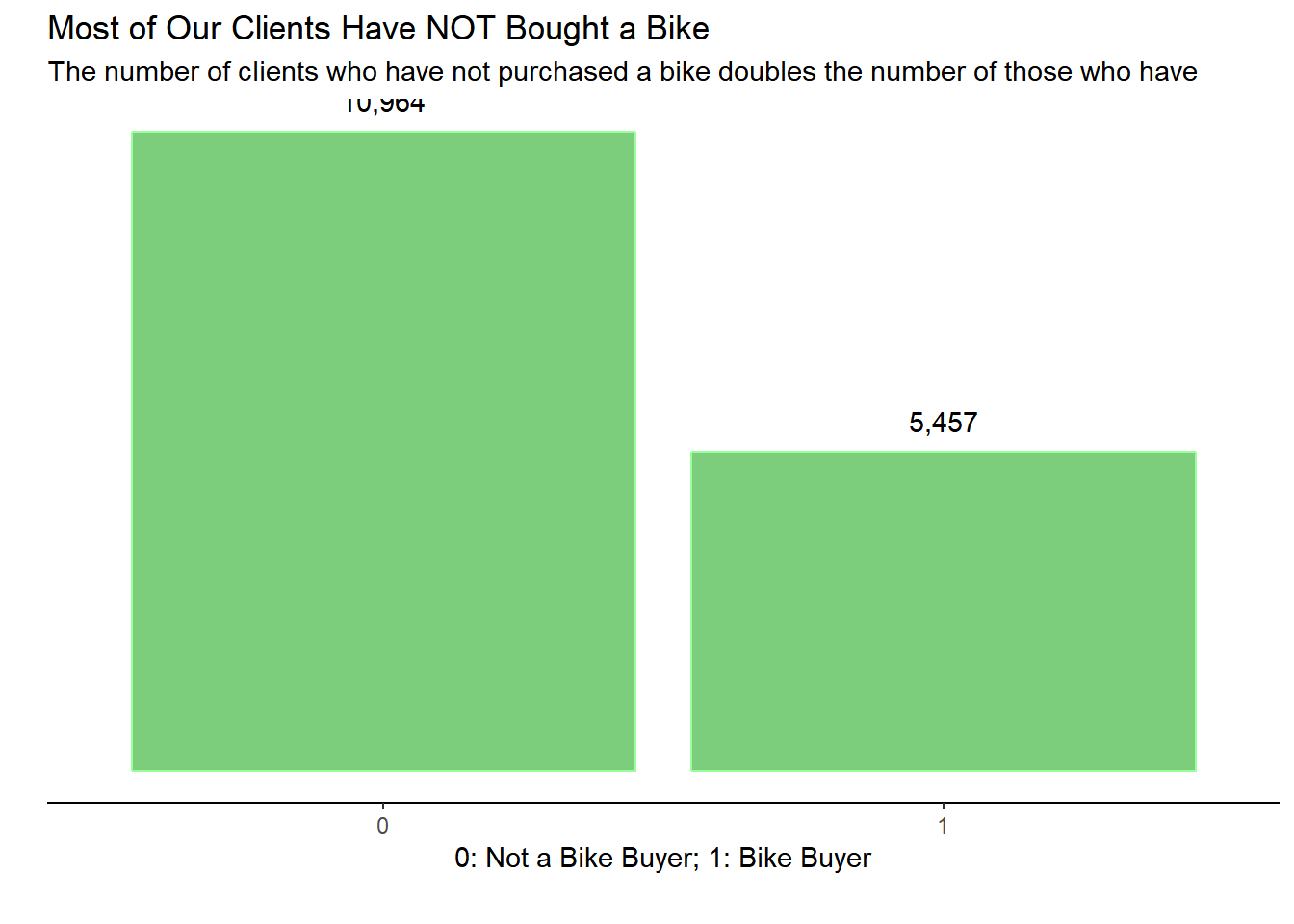
The company is interested in raising the number of clients who buy bikes; let’s check our BikeBuyer column for insights.

ggplot(data_clean, 
       aes(x = as.factor(BikeBuyer), 
           label=..count..)) +
  geom_histogram(binwidth = .5, 
                 colour   = "palegreen1", 
                 fill     = "palegreen3", 
                 stat     = 'count') +
  labs(title    = "Most of Our Clients Have NOT Bought a Bike", 
       subtitle = "The number of clients who have not purchased a bike doubles the number of those who have", 
       caption  = "", 
       x        = "0: Not a Bike Buyer; 1: Bike Buyer",
       y        = '') + 
  theme_classic() +
  geom_text(stat = 'count', 
            aes(label = comma(..count..), 
            vjust = -1)) +
  scale_y_continuous(breaks = NULL, 
                     labels = comma)

Insight: As we can see in the graph, fewer customers have bought bikes than have not bought bikes. We should consider adveritising our bikes more, rather than just the parts.

Income:

means <- tapply(data_clean$YearlyIncome, INDEX = data_clean$Occupation, FUN = mean) #Gets the mean by group

ggplot(data_clean, 
       aes(x = forcats::fct_reorder(Occupation, YearlyIncome, .fun=median), y = YearlyIncome))  + 
  geom_boxplot( width = .5, 
                fill="palegreen3")  + 
  theme(axis.text.x = element_text(angle = 0, 
                                   vjust = 0.6)) +
  scale_y_continuous(breaks = means,
                     labels = dollar) + 
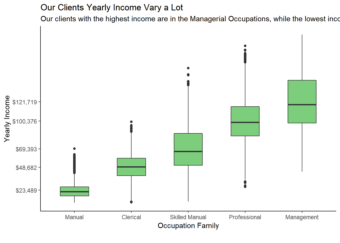
  labs(title    = "Our Clients Yearly Income Vary a Lot", 
       subtitle = "Our clients with the highest income are in the Managerial Occupations, while the lowest income are in the Manual Occupation", 
       caption  = "", 
       x        = "Occupation Family",
       y        = 'Yearly Income') + 
  theme_classic()

Insight: we have clients from all occupational families. Their Yearly Income from lowest to highest is: Manual, Clerical, Skilled Manual, Professional, Management.

Gender

ggplot(data_clean, aes(AveMonthSpend)) +
  geom_density(aes(fill=factor(Gender)), 
                 alpha=0.8) + 
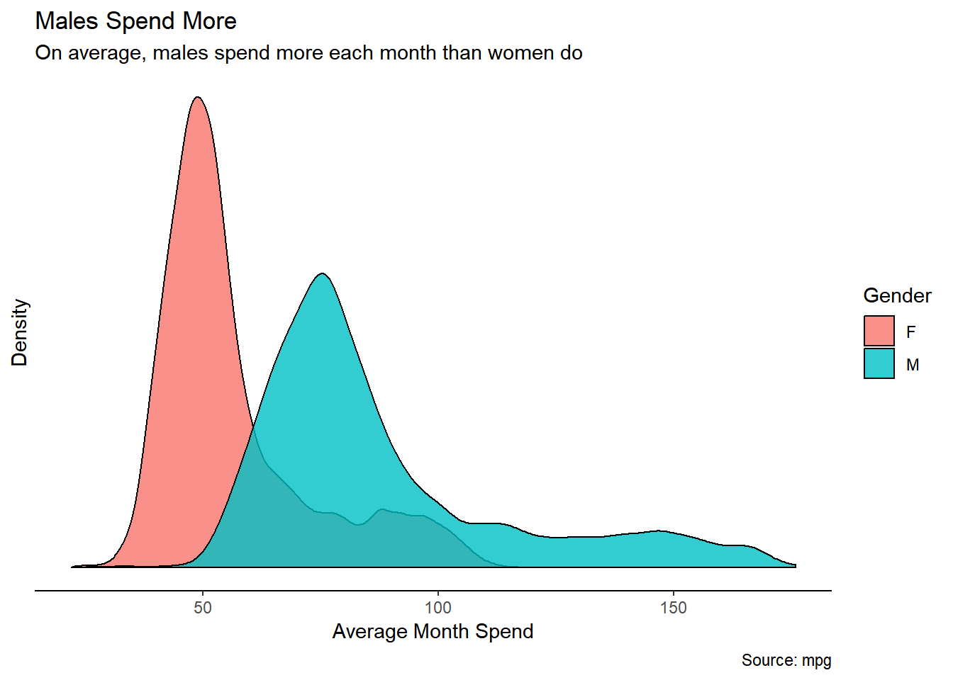
    labs(title = "Males Spend More", 
         subtitle = "On average, males spend more each month than women do",
         caption = "Source: mpg",
         x = "Average Month Spend",
         y = 'Density',
         fill = "Gender") + 
  scale_y_continuous(breaks = NULL) +
  theme_classic()

Insight: Males on average tend to spend more; the “sweet spot” or a range in which both males and females spend equally seems to be “$50-75”; something intersting is that only males spend more than “$120” a month.

Family

ggplot(data_clean, 
       aes(x = MaritalStatus, 
           y = AveMonthSpend))  + 
  geom_bar(stat = "identity", 
           width = .5, 
           aes(fill = Gender))  + 
  theme(axis.text.x = element_text(angle=0, 
                                   vjust=0.6)) + 
  facet_grid(Gender ~ HomeOwnerFlag) +
  scale_y_continuous(labels = dollar) + 
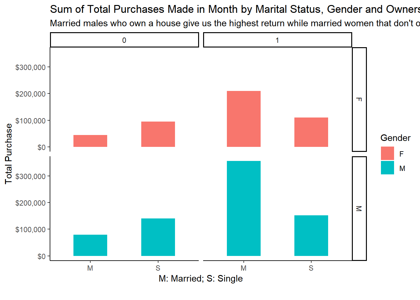
  labs(title    = "Sum of Total Purchases Made in Month by Marital Status, Gender and Ownership of House", 
       subtitle = "Married males who own a house give us the highest return while married women that don't own a house are the lowest", 
       caption  = "", 
       x        = "M: Married; S: Single",
       y        = 'Total Purchase') + 
  theme_classic()

Insight: Married males who own a house give us the highest return while married women that don’t own a house are the lowest